Fieldkit and OpenFTS

The primary use of fieldkit to to help users manipulate the field files generated by OpenFTS.

Writing fields for OpenFTS

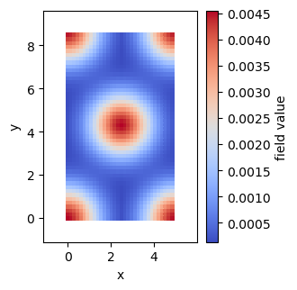
Lets use fieldkit to initialize fields to trap a simulation in the HEX phase. First we will initialize the \(w_-\) field and plot it

import fieldkit as fk
import numpy as np

# initialize a field with the appropriate cell size
npw=(32,48)
Lx = 5.0
Ly = Lx*np.sqrt(3)
h = np.array([[Lx,0],[0,Ly]])
field_wminus = fk.Field(npw=npw,h=h)

fk.add_gaussian(field_wminus,center=(0,0), sigma=1.0)
fk.add_gaussian(field_wminus,center=(0.5*Lx,0.5*Ly), sigma=1.0)

fk.plot(field_wminus,dpi=100)

Now lets randomly initialize the \(w_+\) field

field_wplus = fk.Field(npw=npw,h=h)
field_wplus.data = np.random.random(npw)

Finally we can write the two fields to a file which can be read using OpenFTS

fk.write_to_file('fields_in.dat',[field_wplus, field_wminus])

Writting 2 fields to fields_in.dat

Fieldkit has a number of build-in functions for initializing fields. For example, it is easy to initialize the A15 phase:

npw = (32,32,32)
h = 6.0* np.eye(3)
fields = fk.initialize_phase("A15", npw, h)
fk.plot(fields)

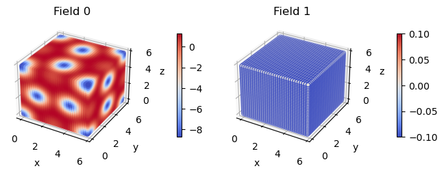
Internally, this is doing nothing more than placing gaussians at the corresponding location of the A15 micelles. Also note that the 2nd field is blank since that is typically the \(w_+\) field.

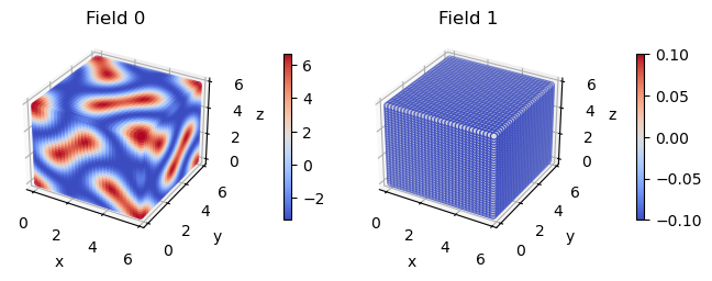
You can also use level-set equations to initialized phases. For example, the double gyroid phase:

npw = (32,32,32)
h = 6.0* np.eye(3)
fields = fk.initialize_phase("double-gyroid", npw, h)
fk.plot(fields)

Reading fields from OpenFTS

2d example

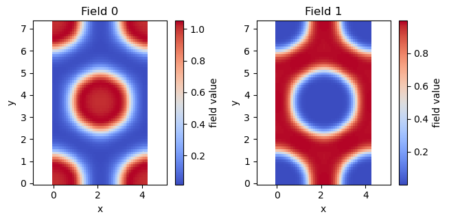
Reading an OpenFTS field file is just as straightforward

fields = fk.read_from_file('density_2d_HEX.dat')

This function returns a list of fields corresponding to each field stored in the field file

fields

[<fieldkit.field.Field at 0x7fe86f017490>,
 <fieldkit.field.Field at 0x7fe86ee55dc0>]

Plotting a list of fields can use the same plot() function as before

fk.plot(fields)

Note: not plotting imaginary part of field 0
Note: not plotting imaginary part of field 1

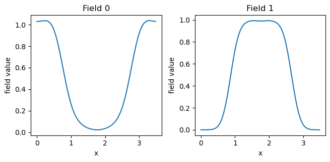
1d example: lamellar phase

Now lets load and plot a 1d field

fields = fk.read_from_file('density_1d_LAM.dat')
fk.plot(fields)

Note: not plotting imaginary part of field 0
Note: not plotting imaginary part of field 1

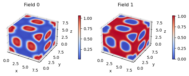
3d example: A15 phase

Finally, lets load and plot the converged A15 phase from OpenFTS

fields = fk.read_from_file('density_3d_A15.dat')
fk.plot(fields)

Note: not plotting imaginary part of field 0
Note: not plotting imaginary part of field 1

The output of fieldkit.plot() is typically sufficient for quick and dirty plotting but is inadequate for publication quality figures. When high-quality images are needed, it is recommended to first write the fields to a .vtk file using fieldkit.write_to_VTK() and then vizualize using paraview.

Check out the next tutorial for how to manipulate field files.